 Mixing
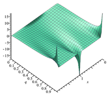
Theta function

Jacobi's original theta function θ1 with u = iπz and with nome q = eiπτ = 0.1e0.1iπ. Conventions are (Mathematica):
θ1(u;q)=2q14∑n=0∞(−1)nqn(n+1)sin(2n+1)u=∑n=−∞n=∞(−1)n−12q(n+12)2e(2n+1)iudisplaystyle beginalignedtheta _1(u;q)&=2q^frac 14sum _n=0^infty (-1)^nq^n(n+1)sin(2n+1)u\&=sum _n=-infty ^n=infty (-1)^n-frac 12q^left(n+frac 12right)^2e^(2n+1)iuendaligned

In mathematics, theta functions are special functions of several complex variables. They are important in many areas, including the theories of Abelian varieties and moduli spaces, and of quadratic forms. They have also been applied to soliton theory. When generalized to a Grassmann algebra, they also appear in quantum field theory.[1]
The most common form of theta function is that occurring in the theory of elliptic functions. With respect to one of the complex variables (conventionally called z), a theta function has a property expressing its behavior with respect to the addition of a period of the associated elliptic functions, making it a quasiperiodic function. In the abstract theory this comes from a line bundle condition of descent.
Contents
1 Jacobi theta function
2 Auxiliary functions
3 Jacobi identities
4 Theta functions in terms of the nome
5 Product representations
6 Integral representations
7 Explicit values
8 Some series identities
9 Zeros of the Jacobi theta functions
10 Relation to the Riemann zeta function
11 Relation to the Weierstrass elliptic function
12 Relation to the q-gamma function
13 Relations to Dedekind eta function
14 Elliptic modulus
15 A solution to the heat equation
16 Relation to the Heisenberg group
17 Generalizations
17.1 Theta series of a Dirichlet character
17.2 Ramanujan theta function
17.3 Riemann theta function
17.4 Poincaré series
18 Notes
19 References
20 Further reading
21 External links
Jacobi theta function

Jacobi theta 1
Jacobi theta 2

Jacobi theta 3

Jacobi theta 4
There are several closely related functions called Jacobi theta functions, and many different and incompatible systems of notation for them.
One Jacobi theta function (named after Carl Gustav Jacob Jacobi) is a function defined for two complex variables z and τ, where z can be any complex number and τ is confined to the upper half-plane, which means it has positive imaginary part. It is given by the formula
- ϑ(z;τ)=∑n=−∞∞exp(πin2τ+2πinz)=1+2∑n=1∞(eπiτ)n2cos(2πnz)=∑n=−∞∞qn2ηndisplaystyle beginalignedvartheta (z;tau )&=sum _n=-infty ^infty exp left(pi in^2tau +2pi inzright)\&=1+2sum _n=1^infty left(e^pi itau right)^n^2cos(2pi nz)=sum _n=-infty ^infty q^n^2eta ^nendaligned

where q = exp(πiτ) and η = exp(2πiz). It is a Jacobi form. If τ is fixed, this becomes a Fourier series for a periodic entire function of z with period 1; in this case, the theta function satisfies the identity
- ϑ(z+1;τ)=ϑ(z;τ).displaystyle vartheta (z+1;tau )=vartheta (z;tau ).

The function also behaves very regularly with respect to its quasi-period τ and satisfies the functional equation
- ϑ(z+a+bτ;τ)=exp(−πib2τ−2πibz)ϑ(z;τ)displaystyle vartheta (z+a+btau ;tau )=exp left(-pi ib^2tau -2pi ibzright),vartheta (z;tau )

where a and b are integers.

Theta function θ1 with different nome q = eiπτ. The black dot in the right-hand picture indicates how q changes with τ.

Theta function θ1 with different nome q = eiπτ. The black dot in the right-hand picture indicates how q changes with τ.
Auxiliary functions
The Jacobi theta function defined above is sometimes considered along with three auxiliary theta functions, in which case it is written with a double 0 subscript:
- ϑ00(z;τ)=ϑ(z;τ)displaystyle vartheta _00(z;tau )=vartheta (z;tau )

The auxiliary (or half-period) functions are defined by
- ϑ01(z;τ)=ϑ(z+12;τ)ϑ10(z;τ)=exp(14πiτ+πiz)ϑ(z+12τ;τ)ϑ11(z;τ)=exp(14πiτ+πi(z+12))ϑ(z+12τ+12;τ).displaystyle beginalignedvartheta _01(z;tau )&=vartheta !left(z+tfrac 12;tau right)\[3pt]vartheta _10(z;tau )&=exp left(tfrac 14pi itau +pi izright)vartheta left(z+tfrac 12tau ;tau right)\[3pt]vartheta _11(z;tau )&=exp left(tfrac 14pi itau +pi ileft(z+tfrac 12right)right)vartheta left(z+tfrac 12tau +tfrac 12;tau right).endaligned
![displaystyle beginalignedvartheta _01(z;tau )&=vartheta !left(z+tfrac 12;tau right)\[3pt]vartheta _10(z;tau )&=exp left(tfrac 14pi itau +pi izright)vartheta left(z+tfrac 12tau ;tau right)\[3pt]vartheta _11(z;tau )&=exp left(tfrac 14pi itau +pi ileft(z+tfrac 12right)right)vartheta left(z+tfrac 12tau +tfrac 12;tau right).endaligned](https://wikimedia.org/api/rest_v1/media/math/render/svg/3cb2997db68ed0c1efa463393856811997d4e439)
This notation follows Riemann and Mumford; Jacobi's original formulation was in terms of the nome q = eiπτ rather than τ. In Jacobi's notation the θ-functions are written:
- θ1(z;q)=−ϑ11(z;τ)θ2(z;q)=ϑ10(z;τ)θ3(z;q)=ϑ00(z;τ)θ4(z;q)=ϑ01(z;τ)displaystyle beginalignedtheta _1(z;q)&=-vartheta _11(z;tau )\theta _2(z;q)&=vartheta _10(z;tau )\theta _3(z;q)&=vartheta _00(z;tau )\theta _4(z;q)&=vartheta _01(z;tau )endaligned

The above definitions of the Jacobi theta functions are by no means unique. See Jacobi theta functions (notational variations) for further discussion.
If we set z = 0 in the above theta functions, we obtain four functions of τ only, defined on the upper half-plane (sometimes called theta constants.) These can be used to define a variety of modular forms, and to parametrize certain curves; in particular, the Jacobi identity is
- ϑ00(0;τ)4=ϑ01(0;τ)4+ϑ10(0;τ)4displaystyle vartheta _00(0;tau )^4=vartheta _01(0;tau )^4+vartheta _10(0;tau )^4

which is the Fermat curve of degree four.
Jacobi identities
Jacobi's identities describe how theta functions transform under the modular group, which is generated by τ ↦ τ + 1 and τ ↦ −1/τ. Equations for the first transform are easily found since adding one to τ in the exponent has the same effect as adding 1/2 to z (n ≡ n2mod 2). For the second, let
- α=(−iτ)12exp(πτiz2).displaystyle alpha =(-itau )^frac 12exp left(frac pi tau iz^2right).

Then
- ϑ00(zτ;−1τ)=αϑ00(z;τ)ϑ01(zτ;−1τ)=αϑ10(z;τ)ϑ10(zτ;−1τ)=αϑ01(z;τ)ϑ11(zτ;−1τ)=−iαϑ11(z;τ).displaystyle beginalignedvartheta _00!left(frac ztau ;frac -1tau right)&=alpha ,vartheta _00(z;tau )quad &vartheta _01!left(frac ztau ;frac -1tau right)&=alpha ,vartheta _10(z;tau )\[3pt]vartheta _10!left(frac ztau ;frac -1tau right)&=alpha ,vartheta _01(z;tau )quad &vartheta _11!left(frac ztau ;frac -1tau right)&=-ialpha ,vartheta _11(z;tau ).endaligned
![displaystyle beginalignedvartheta _00!left(frac ztau ;frac -1tau right)&=alpha ,vartheta _00(z;tau )quad &vartheta _01!left(frac ztau ;frac -1tau right)&=alpha ,vartheta _10(z;tau )\[3pt]vartheta _10!left(frac ztau ;frac -1tau right)&=alpha ,vartheta _01(z;tau )quad &vartheta _11!left(frac ztau ;frac -1tau right)&=-ialpha ,vartheta _11(z;tau ).endaligned](https://wikimedia.org/api/rest_v1/media/math/render/svg/e38521d263e968c6643113cb856744c3d8417638)
Theta functions in terms of the nome
Instead of expressing the Theta functions in terms of z and τ, we may express them in terms of arguments w and the nome q, where w = eπiz and q = eπiτ. In this form, the functions become
- ϑ00(w,q)=∑n=−∞∞(w2)nqn2ϑ01(w,q)=∑n=−∞∞(−1)n(w2)nqn2ϑ10(w,q)=∑n=−∞∞(w2)n+12q(n+12)2ϑ11(w,q)=i∑n=−∞∞(−1)n(w2)n+12q(n+12)2.displaystyle beginalignedvartheta _00(w,q)&=sum _n=-infty ^infty (w^2)^nq^n^2quad &vartheta _01(w,q)&=sum _n=-infty ^infty (-1)^n(w^2)^nq^n^2\[3pt]vartheta _10(w,q)&=sum _n=-infty ^infty (w^2)^n+frac 12q^left(n+frac 12right)^2quad &vartheta _11(w,q)&=isum _n=-infty ^infty (-1)^n(w^2)^n+frac 12q^left(n+frac 12right)^2.endaligned
![displaystyle beginalignedvartheta _00(w,q)&=sum _n=-infty ^infty (w^2)^nq^n^2quad &vartheta _01(w,q)&=sum _n=-infty ^infty (-1)^n(w^2)^nq^n^2\[3pt]vartheta _10(w,q)&=sum _n=-infty ^infty (w^2)^n+frac 12q^left(n+frac 12right)^2quad &vartheta _11(w,q)&=isum _n=-infty ^infty (-1)^n(w^2)^n+frac 12q^left(n+frac 12right)^2.endaligned](https://wikimedia.org/api/rest_v1/media/math/render/svg/db65827472877657a7aa66887c63a13ecd71483a)
We see that the theta functions can also be defined in terms of w and q, without a direct reference to the exponential function. These formulas can, therefore, be used to define the Theta functions over other fields where the exponential function might not be everywhere defined, such as fields of p-adic numbers.
Product representations
The Jacobi triple product (a special case of the Macdonald identities) tells us that for complex numbers w and q with |q| < 1 and w ≠ 0 we have
- ∏m=1∞(1−q2m)(1+w2q2m−1)(1+w−2q2m−1)=∑n=−∞∞w2nqn2.displaystyle prod _m=1^infty left(1-q^2mright)left(1+w^2q^2m-1right)left(1+w^-2q^2m-1right)=sum _n=-infty ^infty w^2nq^n^2.

It can be proven by elementary means, as for instance in Hardy and Wright's An Introduction to the Theory of Numbers.
If we express the theta function in terms of the nome q = eπiτ and w = eπiz then
- ϑ(z;τ)=∑n=−∞∞exp(πiτn2)exp(2πizn)=∑n=−∞∞w2nqn2.displaystyle vartheta (z;tau )=sum _n=-infty ^infty exp(pi itau n^2)exp(2pi izn)=sum _n=-infty ^infty w^2nq^n^2.

We therefore obtain a product formula for the theta function in the form
- ϑ(z;τ)=∏m=1∞(1−exp(2mπiτ))(1+exp((2m−1)πiτ+2πiz))(1+exp((2m−1)πiτ−2πiz)).displaystyle vartheta (z;tau )=prod _m=1^infty big (1-exp(2mpi itau )big )Big (1+exp big ((2m-1)pi itau +2pi izbig )Big )Big (1+exp big ((2m-1)pi itau -2pi izbig )Big ).

In terms of w and q:
- ϑ(z;τ)=∏m=1∞(1−q2m)(1+q2m−1w2)(1+q2m−1w2)=(q2;q2)∞(−w2q;q2)∞(−qw2;q2)∞=(q2;q2)∞θ(−w2q;q2)displaystyle beginalignedvartheta (z;tau )&=prod _m=1^infty left(1-q^2mright)left(1+q^2m-1w^2right)left(1+frac q^2m-1w^2right)\&=left(q^2;q^2right)_infty ,left(-w^2q;q^2right)_infty ,left(-frac qw^2;q^2right)_infty \&=left(q^2;q^2right)_infty ,theta left(-w^2q;q^2right)endaligned

where ( ; )∞ is the q-Pochhammer symbol and θ( ; ) is the q-theta function. Expanding terms out, the Jacobi triple product can also be written
- ∏m=1∞(1−q2m)(1+(w2+w−2)q2m−1+q4m−2),displaystyle prod _m=1^infty left(1-q^2mright)Big (1+left(w^2+w^-2right)q^2m-1+q^4m-2Big ),

which we may also write as
- ϑ(z∣q)=∏m=1∞(1−q2m)(1+2cos(2πz)q2m−1+q4m−2).displaystyle vartheta (zmid q)=prod _m=1^infty left(1-q^2mright)left(1+2cos(2pi z)q^2m-1+q^4m-2right).

This form is valid in general but clearly is of particular interest when z is real. Similar product formulas for the auxiliary theta functions are
- ϑ01(z∣q)=∏m=1∞(1−q2m)(1−2cos(2πz)q2m−1+q4m−2),ϑ10(z∣q)=2q14cos(πz)∏m=1∞(1−q2m)(1+2cos(2πz)q2m+q4m),ϑ11(z∣q)=−2q14sin(πz)∏m=1∞(1−q2m)(1−2cos(2πz)q2m+q4m).displaystyle beginalignedvartheta _01(zmid q)&=prod _m=1^infty left(1-q^2mright)left(1-2cos(2pi z)q^2m-1+q^4m-2right),\[3pt]vartheta _10(zmid q)&=2q^frac 14cos(pi z)prod _m=1^infty left(1-q^2mright)left(1+2cos(2pi z)q^2m+q^4mright),\[3pt]vartheta _11(zmid q)&=-2q^frac 14sin(pi z)prod _m=1^infty left(1-q^2mright)left(1-2cos(2pi z)q^2m+q^4mright).endaligned
![displaystyle beginalignedvartheta _01(zmid q)&=prod _m=1^infty left(1-q^2mright)left(1-2cos(2pi z)q^2m-1+q^4m-2right),\[3pt]vartheta _10(zmid q)&=2q^frac 14cos(pi z)prod _m=1^infty left(1-q^2mright)left(1+2cos(2pi z)q^2m+q^4mright),\[3pt]vartheta _11(zmid q)&=-2q^frac 14sin(pi z)prod _m=1^infty left(1-q^2mright)left(1-2cos(2pi z)q^2m+q^4mright).endaligned](https://wikimedia.org/api/rest_v1/media/math/render/svg/1a2f486ca65bf1df31851e9591220ff601cf6fb0)
Integral representations
The Jacobi theta functions have the following integral representations:
- ϑ00(z;τ)=−i∫i−∞i+∞eiπτu2cos(2uz+πu)sin(πu)du;ϑ01(z;τ)=−i∫i−∞i+∞eiπτu2cos(2uz)sin(πu)du;ϑ10(z;τ)=−ieiz+14iπτ∫i−∞i+∞eiπτu2cos(2uz+πu+πτu)sin(πu)du;ϑ11(z;τ)=eiz+14iπτ∫i−∞i+∞eiπτu2cos(2uz+πτu)sin(πu)du.displaystyle beginalignedvartheta _00(z;tau )&=-iint _i-infty ^i+infty e^ipi tau u^2frac cos(2uz+pi u)sin(pi u)mathrm d u;\[6pt]vartheta _01(z;tau )&=-iint _i-infty ^i+infty e^ipi tau u^2frac cos(2uz)sin(pi u)mathrm d u;\[6pt]vartheta _10(z;tau )&=-ie^iz+frac 14ipi tau int _i-infty ^i+infty e^ipi tau u^2frac cos(2uz+pi u+pi tau u)sin(pi u)mathrm d u;\[6pt]vartheta _11(z;tau )&=e^iz+frac 14ipi tau int _i-infty ^i+infty e^ipi tau u^2frac cos(2uz+pi tau u)sin(pi u)mathrm d u.endaligned
![displaystyle beginalignedvartheta _00(z;tau )&=-iint _i-infty ^i+infty e^ipi tau u^2frac cos(2uz+pi u)sin(pi u)mathrm d u;\[6pt]vartheta _01(z;tau )&=-iint _i-infty ^i+infty e^ipi tau u^2frac cos(2uz)sin(pi u)mathrm d u;\[6pt]vartheta _10(z;tau )&=-ie^iz+frac 14ipi tau int _i-infty ^i+infty e^ipi tau u^2frac cos(2uz+pi u+pi tau u)sin(pi u)mathrm d u;\[6pt]vartheta _11(z;tau )&=e^iz+frac 14ipi tau int _i-infty ^i+infty e^ipi tau u^2frac cos(2uz+pi tau u)sin(pi u)mathrm d u.endaligned](https://wikimedia.org/api/rest_v1/media/math/render/svg/d64804e9cd7ac2b0dbe01eb172d0eaeb0289601a)
Explicit values
See Yi (2004).[2]
- φ(e−πx)=ϑ(0;ix)=θ3(0;e−πx)=∑n=−∞∞e−xπn2φ(e−π)=π4Γ(34)φ(e−2π)=6π+42π42Γ(34)φ(e−3π)=27π+183π43Γ(34)φ(e−4π)=8π4+2π44Γ(34)φ(e−5π)=225π+1005π45Γ(34)φ(e−6π)=32+334+23−274+17284−43⋅243π2861+6−2−36Γ(34)displaystyle beginalignedvarphi (e^-pi x)&=vartheta (0;ix)=theta _3(0;e^-pi x)=sum _n=-infty ^infty e^-xpi n^2\[6pt]varphi left(e^-pi right)&=frac sqrt[4]pi Gamma left(frac 34right)\[6pt]varphi left(e^-2pi right)&=frac sqrt[4]6pi +4sqrt 2pi 2Gamma left(frac 34right)\[6pt]varphi left(e^-3pi right)&=frac sqrt[4]27pi +18sqrt 3pi 3Gamma left(frac 34right)\[6pt]varphi left(e^-4pi right)&=frac sqrt[4]8pi +2sqrt[4]pi 4Gamma left(frac 34right)\[6pt]varphi left(e^-5pi right)&=frac sqrt[4]225pi +100sqrt 5pi 5Gamma left(frac 34right)\[6pt]varphi left(e^-6pi right)&=frac sqrt[3]3sqrt 2+3sqrt[4]3+2sqrt 3-sqrt[4]27+sqrt[4]1728-4cdot sqrt[8]243pi ^26sqrt[6]1+sqrt 6-sqrt 2-sqrt 3;Gamma left(frac 34right)endaligned
![displaystyle beginalignedvarphi (e^-pi x)&=vartheta (0;ix)=theta _3(0;e^-pi x)=sum _n=-infty ^infty e^-xpi n^2\[6pt]varphi left(e^-pi right)&=frac sqrt[4]pi Gamma left(frac 34right)\[6pt]varphi left(e^-2pi right)&=frac sqrt[4]6pi +4sqrt 2pi 2Gamma left(frac 34right)\[6pt]varphi left(e^-3pi right)&=frac sqrt[4]27pi +18sqrt 3pi 3Gamma left(frac 34right)\[6pt]varphi left(e^-4pi right)&=frac sqrt[4]8pi +2sqrt[4]pi 4Gamma left(frac 34right)\[6pt]varphi left(e^-5pi right)&=frac sqrt[4]225pi +100sqrt 5pi 5Gamma left(frac 34right)\[6pt]varphi left(e^-6pi right)&=frac sqrt[3]3sqrt 2+3sqrt[4]3+2sqrt 3-sqrt[4]27+sqrt[4]1728-4cdot sqrt[8]243pi ^26sqrt[6]1+sqrt 6-sqrt 2-sqrt 3;Gamma left(frac 34right)endaligned](https://wikimedia.org/api/rest_v1/media/math/render/svg/b80e5c60d786bafa972d96b734588b8ff8ee88f5)
Some series identities
The next two series identities were proved by István Mező:[3]
- ϑ42(q)=iq14∑k=−∞∞q2k2−kϑ1(2k−12ilnq,q),ϑ42(q)=∑k=−∞∞q2k2ϑ4(klnqi,q).displaystyle beginalignedvartheta _4^2(q)&=iq^frac 14sum _k=-infty ^infty q^2k^2-kvartheta _1left(frac 2k-12iln q,qright),\[6pt]vartheta _4^2(q)&=sum _k=-infty ^infty q^2k^2vartheta _4left(frac kln qi,qright).endaligned
![displaystyle beginalignedvartheta _4^2(q)&=iq^frac 14sum _k=-infty ^infty q^2k^2-kvartheta _1left(frac 2k-12iln q,qright),\[6pt]vartheta _4^2(q)&=sum _k=-infty ^infty q^2k^2vartheta _4left(frac kln qi,qright).endaligned](https://wikimedia.org/api/rest_v1/media/math/render/svg/b8c16f39ab9443e220062eaad77d207fd8ff5cb0)
These relations hold for all 0 < q < 1. Specializing the values of q, we have the next parameter free sums
- πeπ2⋅1Γ2(34)=i∑k=−∞∞eπ(k−2k2)ϑ1(iπ2(2k−1),e−π),π2⋅1Γ2(34)=∑k=−∞∞ϑ4(ikπ,e−π)e2πk2displaystyle beginalignedsqrt frac pi sqrt e^pi 2cdot frac 1Gamma ^2left(frac 34right)&=isum _k=-infty ^infty e^pi left(k-2k^2right)vartheta _1left(frac ipi 2(2k-1),e^-pi right),\[6pt]sqrt frac pi 2cdot frac 1Gamma ^2left(frac 34right)&=sum _k=-infty ^infty frac vartheta _4left(ikpi ,e^-pi right)e^2pi k^2endaligned
![displaystyle beginalignedsqrt frac pi sqrt e^pi 2cdot frac 1Gamma ^2left(frac 34right)&=isum _k=-infty ^infty e^pi left(k-2k^2right)vartheta _1left(frac ipi 2(2k-1),e^-pi right),\[6pt]sqrt frac pi 2cdot frac 1Gamma ^2left(frac 34right)&=sum _k=-infty ^infty frac vartheta _4left(ikpi ,e^-pi right)e^2pi k^2endaligned](https://wikimedia.org/api/rest_v1/media/math/render/svg/8e539c4d92a7653e109301a20da7afb6e1325a1f)
Zeros of the Jacobi theta functions
All zeros of the Jacobi theta functions are simple zeros and are given by the following:
- ϑ(z,τ)=ϑ3(z,τ)=0⟺z=m+nτ+12+τ2ϑ1(z,τ)=0⟺z=m+nτϑ2(z,τ)=0⟺z=m+nτ+12ϑ4(z,τ)=0⟺z=m+nτ+τ2displaystyle beginalignedvartheta (z,tau )=vartheta _3(z,tau )&=0quad &Longleftrightarrow &&quad z&=m+ntau +frac 12+frac tau 2\[3pt]vartheta _1(z,tau )&=0quad &Longleftrightarrow &&quad z&=m+ntau \[3pt]vartheta _2(z,tau )&=0quad &Longleftrightarrow &&quad z&=m+ntau +frac 12\[3pt]vartheta _4(z,tau )&=0quad &Longleftrightarrow &&quad z&=m+ntau +frac tau 2endaligned
![displaystyle beginalignedvartheta (z,tau )=vartheta _3(z,tau )&=0quad &Longleftrightarrow &&quad z&=m+ntau +frac 12+frac tau 2\[3pt]vartheta _1(z,tau )&=0quad &Longleftrightarrow &&quad z&=m+ntau \[3pt]vartheta _2(z,tau )&=0quad &Longleftrightarrow &&quad z&=m+ntau +frac 12\[3pt]vartheta _4(z,tau )&=0quad &Longleftrightarrow &&quad z&=m+ntau +frac tau 2endaligned](https://wikimedia.org/api/rest_v1/media/math/render/svg/b0a46570a37094335d8daa1755155d36ad316b6d)
where m, n are arbitrary integers.
Relation to the Riemann zeta function
The relation
- ϑ(0;−1τ)=(−iτ)12ϑ(0;τ)displaystyle vartheta left(0;-frac 1tau right)=(-itau )^frac 12vartheta (0;tau )

was used by Riemann to prove the functional equation for the Riemann zeta function, by means of the Mellin transform
- Γ(s2)π−s2ζ(s)=12∫0∞(ϑ(0;it)−1)ts2dttdisplaystyle Gamma left(frac s2right)pi ^-frac s2zeta (s)=frac 12int _0^infty big (vartheta (0;it)-1big )t^frac s2frac mathrm d tt

which can be shown to be invariant under substitution of s by 1 − s. The corresponding integral for z ≠ 0 is given in the article on the Hurwitz zeta function.
Relation to the Weierstrass elliptic function
The theta function was used by Jacobi to construct (in a form adapted to easy calculation) his elliptic functions as the quotients of the above four theta functions, and could have been used by him to construct Weierstrass's elliptic functions also, since
- ℘(z;τ)=−(logϑ11(z;τ))″+cdisplaystyle wp (z;tau )=-big (log vartheta _11(z;tau )big )''+c

where the second derivative is with respect to z and the constant c is defined so that the Laurent expansion of ℘(z) at z = 0 has zero constant term.
Relation to the q-gamma function
The fourth theta function – and thus the others too – is intimately connected to the Jackson q-gamma function via the relation[4]
- (Γq2(x)Γq2(1−x))−1=q2x(1−x)(q−2;q−2)∞3(q2−1)ϑ4(12i(1−2x)logq,1q).displaystyle left(Gamma _q^2(x)Gamma _q^2(1-x)right)^-1=frac q^2x(1-x)left(q^-2;q^-2right)_infty ^3left(q^2-1right)vartheta _4left(frac 12i(1-2x)log q,frac 1qright).

Relations to Dedekind eta function
Let η(τ) be the Dedekind eta function, and the argument of the theta function as the nome q = eπiτ. Then,
- θ2(0,q)=ϑ10(0;τ)=2η2(2τ)η(τ),θ3(0,q)=ϑ00(0;τ)=η5(τ)η2(12τ)η2(2τ)=η2(12(τ+1))η(τ+1),θ4(0,q)=ϑ01(0;τ)=η2(12τ)η(τ),displaystyle beginalignedtheta _2(0,q)=vartheta _10(0;tau )&=frac 2eta ^2(2tau )eta (tau ),\[3pt]theta _3(0,q)=vartheta _00(0;tau )&=frac eta ^5(tau )eta ^2left(frac 12tau right)eta ^2(2tau )=frac eta ^2left(frac 12(tau +1)right)eta (tau +1),\[3pt]theta _4(0,q)=vartheta _01(0;tau )&=frac eta ^2left(frac 12tau right)eta (tau ),endaligned
![displaystyle beginalignedtheta _2(0,q)=vartheta _10(0;tau )&=frac 2eta ^2(2tau )eta (tau ),\[3pt]theta _3(0,q)=vartheta _00(0;tau )&=frac eta ^5(tau )eta ^2left(frac 12tau right)eta ^2(2tau )=frac eta ^2left(frac 12(tau +1)right)eta (tau +1),\[3pt]theta _4(0,q)=vartheta _01(0;tau )&=frac eta ^2left(frac 12tau right)eta (tau ),endaligned](https://wikimedia.org/api/rest_v1/media/math/render/svg/51aa288fda023bcc1b7d82366605089d3abd4800)
and,
- θ2(0,q)θ3(0,q)θ4(0,q)=2η3(τ).displaystyle theta _2(0,q),theta _3(0,q),theta _4(0,q)=2eta ^3(tau ).

See also the Weber modular functions.
Elliptic modulus
The elliptic modulus is
- k(τ)=ϑ10(0,τ)2ϑ00(0,τ)2displaystyle k(tau )=frac vartheta _10(0,tau )^2vartheta _00(0,tau )^2

and the complementary elliptic modulus is
- k′(τ)=ϑ01(0,τ)2ϑ00(0,τ)2displaystyle k'(tau )=frac vartheta _01(0,tau )^2vartheta _00(0,tau )^2

A solution to the heat equation
The Jacobi theta function is the fundamental solution of the one-dimensional heat equation with spatially periodic boundary conditions.[5] Taking z = x to be real and τ = it with t real and positive, we can write
- ϑ(x,it)=1+2∑n=1∞exp(−πn2t)cos(2πnx)displaystyle vartheta (x,it)=1+2sum _n=1^infty exp left(-pi n^2tright)cos(2pi nx)

which solves the heat equation
- ∂∂tϑ(x,it)=14π∂2∂x2ϑ(x,it).displaystyle frac partial partial tvartheta (x,it)=frac 14pi frac partial ^2partial x^2vartheta (x,it).

This theta-function solution is 1-periodic in x, and as t → 0 it approaches the periodic delta function, or Dirac comb, in the sense of distributions
limt→0ϑ(x,it)=∑n=−∞∞δ(x−n)displaystyle lim _trightarrow 0vartheta (x,it)=sum _n=-infty ^infty delta (x-n).
General solutions of the spatially periodic initial value problem for the heat equation may be obtained by convolving the initial data at t = 0 with the theta function.
Relation to the Heisenberg group
The Jacobi theta function is invariant under the action of a discrete subgroup of the Heisenberg group. This invariance is presented in the article on the theta representation of the Heisenberg group.
Generalizations
If F is a quadratic form in n variables, then the theta function associated with F is
- θF(z)=∑m∈Zne2πizF(m)displaystyle theta _F(z)=sum _min mathbb Z ^ne^2pi izF(m)

with the sum extending over the lattice of integers ℤn. This theta function is a modular form of weight n/2 (on an appropriately defined subgroup) of the modular group. In the Fourier expansion,
- θ^F(z)=∑k=0∞RF(k)e2πikz,displaystyle hat theta _F(z)=sum _k=0^infty R_F(k)e^2pi ikz,

the numbers RF(k) are called the representation numbers of the form.
Theta series of a Dirichlet character
For χdisplaystyle chi 


- θχ(z)=12∑n=−∞∞χ(n)nνe2iπn2zdisplaystyle theta _chi (z)=frac 12sum _n=-infty ^infty chi (n)n^nu e^2ipi n^2z

is a weight 12+νdisplaystyle frac 12+nu 


θχ(az+bcz+d)=χ(d)(−1d)ν(θ1(az+bcz+d)θ1(z))1+2νθχ(z)displaystyle theta _chi left(frac az+bcz+dright)=chi (d)left(frac -1dright)^nu left(frac theta _1left(frac az+bcz+dright)theta _1(z)right)^1+2nu theta _chi (z)whenever a,b,c,d∈Z4,ad−bc=1,c≡0mod4q2displaystyle a,b,c,din mathbb Z ^4,ad-bc=1,cequiv 0bmod 4q^2
[6].
Ramanujan theta function
Riemann theta function
Let
- Hn=F∈M(n,C)displaystyle mathbb H _n=leftFin M(n,mathbb C ),big ,F=F^mathsf T,,,operatorname Im F>0right

the set of symmetric square matrices whose imaginary part is positive definite. ℍn is called the Siegel upper half-space and is the multi-dimensional analog of the upper half-plane. The n-dimensional analogue of the modular group is the symplectic group Sp(2n,ℤ); for n = 1, Sp(2,ℤ) = SL(2,ℤ). The n-dimensional analogue of the congruence subgroups is played by
- kerSp(2n,Z)→Sp(2n,Z/kZ).displaystyle ker big operatorname Sp (2n,mathbb Z )rightarrow operatorname Sp (2n,mathbb Z /kmathbb Z )big .

Then, given τ ∈ ℍn, the Riemann theta function is defined as
- θ(z,τ)=∑m∈Znexp(2πi(12mTτm+mTz)).displaystyle theta (z,tau )=sum _min mathbb Z ^nexp bigg (2pi ileft(tfrac 12m^mathsf Ttau m+m^mathsf Tzright)bigg ).

Here, z ∈ ℂn is an n-dimensional complex vector, and the superscript T denotes the transpose. The Jacobi theta function is then a special case, with n = 1 and τ ∈ ℍ where ℍ is the upper half-plane.
The Riemann theta converges absolutely and uniformly on compact subsets of ℂn × ℍn.
The functional equation is
- θ(z+a+τb,τ)=exp2πi(−bTz−12bTτb)θ(z,τ)displaystyle theta (z+a+tau b,tau )=exp 2pi ileft(-b^mathsf Tz-tfrac 12b^mathsf Ttau bright)theta (z,tau )

which holds for all vectors a, b ∈ ℤn, and for all z ∈ ℂn and τ ∈ ℍn.
Poincaré series
The Poincaré series generalizes the theta series to automorphic forms with respect to arbitrary Fuchsian groups.
Notes
^ Tyurin, Andrey N. (30 October 2002). "Quantization, Classical and Quantum Field Theory and Theta-Functions". arXiv:math/0210466v1. Bibcode:2002math.....10466T..mw-parser-output cite.citationfont-style:inherit.mw-parser-output qquotes:"""""""'""'".mw-parser-output code.cs1-codecolor:inherit;background:inherit;border:inherit;padding:inherit.mw-parser-output .cs1-lock-free abackground:url("//upload.wikimedia.org/wikipedia/commons/thumb/6/65/Lock-green.svg/9px-Lock-green.svg.png")no-repeat;background-position:right .1em center.mw-parser-output .cs1-lock-limited a,.mw-parser-output .cs1-lock-registration abackground:url("//upload.wikimedia.org/wikipedia/commons/thumb/d/d6/Lock-gray-alt-2.svg/9px-Lock-gray-alt-2.svg.png")no-repeat;background-position:right .1em center.mw-parser-output .cs1-lock-subscription abackground:url("//upload.wikimedia.org/wikipedia/commons/thumb/a/aa/Lock-red-alt-2.svg/9px-Lock-red-alt-2.svg.png")no-repeat;background-position:right .1em center.mw-parser-output .cs1-subscription,.mw-parser-output .cs1-registrationcolor:#555.mw-parser-output .cs1-subscription span,.mw-parser-output .cs1-registration spanborder-bottom:1px dotted;cursor:help.mw-parser-output .cs1-hidden-errordisplay:none;font-size:100%.mw-parser-output .cs1-visible-errorfont-size:100%.mw-parser-output .cs1-subscription,.mw-parser-output .cs1-registration,.mw-parser-output .cs1-formatfont-size:95%.mw-parser-output .cs1-kern-left,.mw-parser-output .cs1-kern-wl-leftpadding-left:0.2em.mw-parser-output .cs1-kern-right,.mw-parser-output .cs1-kern-wl-rightpadding-right:0.2em
^ Yi, Jinhee (2004). "Theta-function identities and the explicit formulas for theta-function and their applications". Journal of Mathematical Analysis and Applications. 292: 381–400. doi:10.1016/j.jmaa.2003.12.009.
^ Mező, István (2013), "Duplication formulae involving Jacobi theta functions and Gosper's q-trigonometric functions", Proceedings of the American Mathematical Society, 141 (7): 2401–2410, doi:10.1090/s0002-9939-2013-11576-5
^ Mező, István (2012). "A q-Raabe formula and an integral of the fourth Jacobi theta function". Journal of Number Theory. 133 (2): 692–704. doi:10.1016/j.jnt.2012.08.025.
^ Ohyama, Yousuke (1995). "Differential relations of theta functions". Osaka Journal of Mathematics. 32 (2): 431–450. ISSN 0030-6126.
^ Shimura, On modular forms of half integral weight
References
Abramowitz, Milton; Stegun, Irene A. (1964). Handbook of Mathematical Functions. New York: Dover Publications. sec. 16.27ff. ISBN 0-486-61272-4.
Akhiezer, Naum Illyich (1990) [1970]. Elements of the Theory of Elliptic Functions. AMS Translations of Mathematical Monographs. 79. Providence, RI: AMS. ISBN 0-8218-4532-2.
Farkas, Hershel M.; Kra, Irwin (1980). Riemann Surfaces. New York: Springer-Verlag. ch. 6. ISBN 0-387-90465-4.. (for treatment of the Riemann theta)
Hardy, G. H.; Wright, E. M. (1959). An Introduction to the Theory of Numbers (4th ed.). Oxford: Clarendon Press.
Mumford, David (1983). Tata Lectures on Theta I. Boston: Birkhauser. ISBN 3-7643-3109-7.
Pierpont, James (1959). Functions of a Complex Variable. New York: Dover Publications.
Rauch, Harry E.; Farkas, Hershel M. (1974). Theta Functions with Applications to Riemann Surfaces. Baltimore: Williams & Wilkins. ISBN 0-683-07196-3.
Reinhardt, William P.; Walker, Peter L. (2010), "Theta Functions", in Olver, Frank W. J.; Lozier, Daniel M.; Boisvert, Ronald F.; Clark, Charles W., NIST Handbook of Mathematical Functions, Cambridge University Press, ISBN 978-0521192255, MR 2723248
Whittaker, E. T.; Watson, G. N. (1927). A Course in Modern Analysis (4th ed.). Cambridge: Cambridge University Press. ch. 21.
(history of Jacobi's θ functions)
Further reading
Farkas, Hershel M. (2008). "Theta functions in complex analysis and number theory". In Alladi, Krishnaswami. Surveys in Number Theory. Developments in Mathematics. 17. Springer-Verlag. pp. 57–87. ISBN 978-0-387-78509-7. Zbl 1206.11055.
Schoeneberg, Bruno (1974). "IX. Theta series". Elliptic modular functions. Die Grundlehren der mathematischen Wissenschaften. 203. Springer-Verlag. pp. 203–226. ISBN 3-540-06382-X.- Ackerman, M. Math. Ann. (1979) 244: 75. "On the Generating Functions of Certain Eisenstein Series" Springer-Verlag
External links
Moiseev Igor. "Elliptic functions for Matlab and Octave".
This article incorporates material from Integral representations of Jacobi theta functions on PlanetMath, which is licensed under the Creative Commons Attribution/Share-Alike License.
Authority control |
|
|---|


Comments
Post a Comment